
Bagua is a deep learning training acceleration framework for PyTorch developed by AI platform@Kuaishou Technology and DS3 Lab@ETH. Bagua currently supports:
- Advanced Distributed Training Algorithms: Users can extend the training on a single GPU to multi-GPUs (may across multiple machines) by simply adding a few lines of code (optionally in elastic mode). One prominent feature of Bagua is to provide a flexible system abstraction that supports state-of-the-art system relaxation techniques of distributed training. So far, Bagua has integrated communication primitives including
- Centralized Synchronous Communication (e.g. Gradient AllReduce)
- Decentralized Synchronous Communication (e.g. Decentralized SGD)
- Low Precision Communication (e.g. ByteGrad)
- Asynchronous Communication (e.g. Async Model Average)
- Cached Dataset: When samples in a dataset need tedious preprocessing, or reading the dataset itself is slow, they could become a major bottleneck of the whole training process. Bagua provides cached dataset to speedup this process by caching data samples in memory, so that reading these samples after the first time can be much faster.
- TCP Communication Acceleration (Bagua-Net): Bagua-Net is a low level communication acceleration feature provided by Bagua. It can greatly improve the throughput of AllReduce on TCP network. You can enable Bagua-Net optimization on any distributed training job that uses NCCL to do GPU communication (this includes PyTorch-DDP, Horovod, DeepSpeed, and more).
- Performance Autotuning: Bagua can automatically tune system parameters to achieve the highest throughput.
- Generic Fused Optimizer: Bagua provides generic fused optimizer which improve the performance of optimizers by fusing the optimizer
.step()operation on multiple layers. It can be applied to arbitrary PyTorch optimizer, in contrast to NVIDIA Apex's approach, where only some specific optimizers are implemented. - Load Balanced Data Loader: When the computation complexity of samples in training data are different, for example in NLP and speech tasks, where each sample have different lengths, distributed training throughput can be greatly improved by using Bagua's load balanced data loader, which distributes samples in a way that each worker's workload are similar.
Its effectiveness has been validated in various scenarios and models, including VGG and ResNet on ImageNet, Bert Large, and multiple huge scale industrial applications at Kuaishou such as
- the recommendation system supporting model training with dozens of TB parameters,
- video/image understanding with >1 billion images/videos,
- ASR with TB level datasets,
- etc.
Performance
For more comprehensive and up to date results, refer to Bagua benchmark page.
Cite Bagua
@misc{gan2021bagua,
      title={BAGUA: Scaling up Distributed Learning with System Relaxations},
      author={Shaoduo Gan and Xiangru Lian and Rui Wang and Jianbin Chang and Chengjun Liu and Hongmei Shi and Shengzhuo Zhang and Xianghong Li and Tengxu Sun and Jiawei Jiang and Binhang Yuan and Sen Yang and Ji Liu and Ce Zhang},
      year={2021},
      eprint={2107.01499},
      archivePrefix={arXiv},
      primaryClass={cs.LG}
}
Links
Installation
Installing Bagua
Wheels (precompiled binary packages) are available for Linux (x86_64). Package names are different depending on your CUDA Toolkit version (CUDA Toolkit version is shown in nvcc --version).
| CUDA Toolkit version | Installation command |
|---|---|
| >= v10.2 | pip install bagua-cuda102 |
| >= v11.1 | pip install bagua-cuda111 |
| >= v11.3 | pip install bagua-cuda113 |
| >= v11.5 | pip install bagua-cuda115 |
| >= v11.6 | pip install bagua-cuda116 |
Add --pre to pip install commands to install pre-release (development) versions.
Install from source
To install Bagua by compiling from source code on your machine, you need the following dependencies installed on your system:
- CUDA Toolkit, with CUDA version >= 10.1
- Rust Compiler
- MPI >= 3.0, for example Open MPI
- hwloc >= 2.0
- CMake >= 3.17
- Python >= 3.7
We provide an automatic installation script for Ubuntu. Just run the following command to install Bagua and above libraries (except for CUDA, you should always install CUDA by yourself):
curl -Ls https://raw.githubusercontent.com/BaguaSys/bagua/master/install.sh | sudo bash
Run the following commands to install Bagua (source code packages, which will be compiled on your machine).
# release version
python3 -m pip install bagua --upgrade

# develop version (git master)
python3 -m pip install --pre bagua --upgrade
Use Docker image
We provide Docker image with Bagua installed based on official PyTorch images. You can find them on DockerHub.
Getting Started
Using Bagua is similar to using other distributed training libraries like PyTorch DDP and Horovod.
Migrate from your existing single GPU training code
To use Bagua, you need make the following changes on your training code:
First, import bagua:
import bagua.torch_api as bagua
Then initialize Bagua's process group:
torch.cuda.set_device(bagua.get_local_rank())
bagua.init_process_group()
Then, use torch's distributed sampler for your data loader:
train_dataset = ...
test_dataset = ...

train_sampler = torch.utils.data.distributed.DistributedSampler(train_dataset,
    num_replicas=bagua.get_world_size(), rank=bagua.get_rank())

train_loader = torch.utils.data.DataLoader(
    train_dataset,
    batch_size=batch_size,
    shuffle=(train_sampler is None),
    sampler=train_sampler,
)

test_loader = torch.utils.data.DataLoader(test_dataset, ...)
Finally, wrap you model and optimizer with bagua by adding one line of code to your original script:
def main():
    args = parse_args()
    # define your model and optimizer
    model = MyNet().to(args.device)
    optimizer = torch.optim.SGD(model.parameters(), lr=args.lr)
    # transform to Bagua wrapper
    from bagua.torch_api.algorithms import gradient_allreduce
    model = model.with_bagua(
        [optimizer], gradient_allreduce.GradientAllReduceAlgorithm()
    )

    # train the model over the dataset
    for epoch in range(args.epochs):
        for b_idx, (inputs, targets) in enumerate(train_loader):
            outputs = model(inputs)
            loss = torch.nn.CrossEntropyLoss(outputs, targets)
            optimizer.zero_grad()
            loss.backward()
            optimizer.step()
More examples can be found here.
Launch job
Bagua has a built-in tool bagua.distributed.launch to launch jobs, whose usage is similar to Pytorch torch.distributed.launch.
We introduce how to start distributed training in the following sections.
Single node multi-process training
python -m bagua.distributed.launch --nproc_per_node=8 \
  your_training_script.py (--arg1 --arg2 ...)
Multi-node multi-process training (e.g. two nodes)
Method 1: run command on each node
Node 1: (IP: 192.168.1.1, and has a free port: 1234)
python -m bagua.distributed.launch --nproc_per_node=8 --nnodes=2 --node_rank=0 --master_addr="192.168.1.1" --master_port=1234 your_training_script.py (--arg1 --arg2 ...)
Node 2:
python -m bagua.distributed.launch --nproc_per_node=8 --nnodes=2 --node_rank=1 --master_addr="192.168.1.1" --master_port=1234 your_training_script.py (--arg1 --arg2 ...)
Tips:
If you need some preprocessing work, you can include them in your bash script and launch job by adding
--no_pythonto your command.python -m bagua.distributed.launch --no_python --nproc_per_node=8 bash your_bash_script.sh
Method 2: run command on a single node providing a host list
If the ssh service is available with passwordless login on each node, we can launch a distributed job on a single node with a similar syntax as mpirun.
Bagua provides a program baguarun. For the multi-node training example above, the command to start with bagurun looks like:
baguarun --host_list NODE_1_HOST:NODE_1_SSH_PORT,NODE_2_HOST:NODE_2_SSH_PORT \
                --nproc_per_node=NUM_GPUS_YOU_HAVE --master_port=1234 \
                YOUR_TRAINING_SCRIPT.py (--arg1 --arg2 --arg3 and all other arguments of your training script)
Algorithms
Bagua thrives on the diversity of distributed learning algorithms. The great flexibility of the system makes it possible to smoothly incorporate various of SOTA algorithms while providing automatic optimizations for the performance during the execution. For the end user, Bagua provides a wide range of choices of algorithms, which she can easily try out for her tasks. For the algorithm developer, Bagua is a playground where she can be just focused on the algorithm itself (e.g., the logic and control) without reinventing the wheels (e.g., communication primitives and system optimizations) across different algorithms.
In the following tutorials, we will describe several algorithms that have already been implemented within Bagua, including the main ideas of each algorithm and their usage in specific examples. Then we are going to demonstrate how to add a new algorithm into Bagua.
We welcome contributions to add more algorithms!
Gradient AllReduce
The Gradient AllReduce algorithm is a popular synchronous data-parallel distributed algorithm. It is the algorithm implemented in most existing solutions such as PyTorch DistributedDataParallel, Horovod, and TensorFlow Mirrored Strategy.
With this algorithm, each worker does the following steps in each iteration.
- Compute the gradient using a minibatch.
- Compute the mean of the gradients on all workers by using the AllReduce collective.
- Update the model with the averaged gradient.
In Bagua, this algorithm is supported via the GradientAllReduce algorithm
class. The performance of the GradientAllReduce implementation in Bagua
should be faster than PyTorch DDP and Horovod in most cases.
Bagua supports additional optimizations such as hierarchical communication that
can be configured when instantiating the GradientAllReduce class. They can
further speeds up Bagua in certain scenarios, for example
when the inter-machine network is a bottleneck.
Example usage
A complete example of running Gradient AllReduce can be found at Bagua examples
with --algorithm gradient_allreduce command line argument.
You need to initialize the Bagua algorithm with (see API documentation for what parameters you can customize):
from bagua.torch_api.algorithms import gradient_allreduce
algorithm = gradient_allreduce.GradientAllReduceAlgorithm()
Then decorate your model with:
model = model.with_bagua([optimizer], algorithm)
ByteGrad
Overview
Large scale distributed training requires significant communication cost, which is especially true for large models. For example in traditional synchronous distributed setup with AllReduce to synchronize gradients (which is the case for many libraries, such as Horovod and PyTorch DDP), in each iteration of the training process, the gradient, whose size is equal to the model size, needs to be sent and received on each worker. Such communication cost soon becomes the training bottleneck in many scenarios.
There are many existing papers about how to apply model/gradient compression to save this communication cost. Bagua provides a built-in gradient compression algorithm called ByteGrad, which compresses the gradient floats to 8bit bytes before communication. This saves 3/4 of the original cost. It implements high accuracy min-max quantization operator with optimized CUDA kernels, and hierarchical communication. This makes it much faster (about 50% faster in our benchmark) than other compression implementations in existing frameworks (such as PyTorch PowerSGD) and in the same number of epochs ByteGrad converges similar to full precision algorithms on most tasks.
For comparison with other algorithms (may or may not be compression algorithms), refer to benchmark page.
Algorithm
ByteGrad does the following steps in each iteration. Assume we have nodes and each node has GPUs.
- Calculate gradient on the -th node's -th GPU for all
- The first GPU on each node does a reduce operation to compute the average of all GPUs' gradients on the same node, defined as for the -th node
- The first GPU on -th node quantize the gradient with a quantization function : , for all . Then each node exchange the quantized version between nodes so that each node has the average of all
- The first GPU on each node broadcast the average of all s to every other GPU on the same node, and all GPUs on all workers use this quantized average to update model
The quantization function calculates the minimum value and maximum value of its input, and the split into evenly spaced 256 intervals. Then represent each element of its input by a 8bit integer representing which interval the original element is in.
Example usage
A complete example of running ByteGrad can be found at Bagua examples
with --algorithm bytegrad command line argument.
You need to initialize the Bagua algorithm with (see API documentation for what parameters you can customize):
from bagua.torch_api.algorithms import bytegrad
algorithm = bytegrad.ByteGradAlgorithm()
Then decorate your model with:
model = model.with_bagua([optimizer], algorithm)
Decentralized SGD
Overview of decentralized training
Decentralized SGD is a data-parallel distributed learning algorithm that removes the requirement of a centralized global model among all workers, which makes it quite different from Allreduce-based or Parameter Server-based algorithms regarding the communication pattern. With decentralized SGD, each worker only needs to exchange data with one or a few specific workers, instead of aggregating data globally. Therefore, decentralized communication has much fewer communication connections than Allreduce, and a more balanced communication overhead than Parameter Server. Although decentralized SGD may lead to different models on each worker, it has been proved in theory that the convergence rate of the decentralized SGD algorithm is the same as its centralized counterpart. You can find the detailed analysis about decentralized SGD in our paper.
Decentralized training algorithms
Currently, there are lots of decentralized training algorithms being proposed every now and then. These amazing works are focused on different aspects of decentralized training, like peer selection, data compression, asynchronization and so on, and provide many promising insights. So far Bagua has incorporated two basic decentralized algorithms, i.e., Decentralized SGD and Low Precision Decentralized SGD. With Bagua's automatic system support for decentralization, we are expecting to see increasingly more decentralized algorithms being implemented in the near future.
Decentralized SGD
Now we are going to describe the decentralized SGD algorithm implemented in Bagua. Let's assume the number of workers is , the model parameters on worker is . Each worker is able to send or receive data directly from any other workers. In each iteration , the algorithm repeats the following steps:
- Each worker calculate the local gradients of iteration : .
- Average the local model with its selected peer's model (denote as ), i.e.,
- Update the averaged model with the local gradients,
In step 2, we adopt a strategy to select a peer for each worker in each iteration, such that all workers are properly paired and the data exchanging is efficient in the sense that each worker could exchange data with a different peer between iterations. In short, our strategy evenly split workers into two groups, and dynamically pair workers between two groups, varying from iteration to iteration.
Communication overhead
The communication overhead of decentralized SGD is highly related to the degree of network, i.e., the number of connections a worker has to other workers. Different topologies or strategies will lead to different degrees of the network. It's obvious that the Decentralized SGD algorithm we described before has a network degree of 1. Therefore, in each iteration, a worker only needs to build one connection with one worker to exchange one time of the model size. We compare the communication complexities of different communication patterns regarding the latency and bandwidth of the busiest node.
| Algorithm | Latency complexity | Bandwidth complexity |
|---|---|---|
| Allreduce (Ring) | ||
| Parameter Server | ||
| Decentralized SGD in Bagua |
Benchmark
Given the optimal communication complexity of Decentralized SGD, it can be much faster than its centralized counterparts during the training, especially when the network is slow. We provide some benchmark results here to compare the performance of Decentralized SGD of Bagua with other SOTA systems.
Example usage
A complete example of running Decentralized SGD can be found at Bagua examples
with --algorithm decentralized command line argument.
You need to initialize the Bagua algorithm with (see API documentation for what parameters you can customize):
from bagua.torch_api.algorithms import decentralized
algorithm = decentralized.DecentralizedAlgorithm()
Then decorate your model with:
model = model.with_bagua([optimizer], algorithm)
Low Precision Decentralized SGD
Overview
As the name suggests, low precision decentralized SGD combines decentralized training and quantized training together. It follows the framework of decentralized SGD that each worker does not need to aggregate data globally, but to exchange data with few workers, more specifically, its peers. Thus this algorithm has similar communication overhead with decentralized SGD. The latency complexity and bandwidth complexity of low precision decentralized SGD are both , where is the number of peers. This is consistent with our analysis in decentralized SGD, where we consider a special case that each worker has only one peer.
With communication compression, low precision decentralized SGD can reduce communication overhead further. It should be noted that data exchanged between workers are not compressed local models, but the compressed differences of local models between two successive iterations. In this way, the low precision decentralized SGD algorithm can achieve the same convergence rate with decentralized SGD, as well as full precision centralized ones. Detailed proof can be found in this paper.
Benefiting from both decentralization and communication compression, low precision decentralized SGD is particular useful in high communication latency and low network bandwidth scenarios.
Algorithm
Assume the number of workers is , and the model parameters on worker is , . Each worker stores model replicas of its connected peers and is able to send data to or receive data from its peers. At each iteration , the algorithm repeats the following steps on each worker :
- Calculate the gradient on worker : .
- Update the local model using local stochastic gradient and the weighted average of its connected peers' replicas:
- Compute the difference , and quantize it into with a quantization function .
- Update the local model with compressed difference,
- Send to its connected peers, and update its connected peers' replicas with compressed differences it received,
The quantization function calculates the minimum value and maximum value of its input, and the split into evenly spaced 256 intervals. Then represent each element of its input by a 8bit integer representing which interval the original element is in.
Each worker stores model replicas of its connected peers, once the peers of a worker is determined, they should not be changed during the whole process.
Example usage
A complete example of running Decentralized SGD can be found at Bagua examples
with --algorithm low_precision_decentralized command line argument.
You need to initialize the Bagua algorithm with (see API documentation for further customization):
from bagua.torch_api.algorithms import decentralized
algorithm = decentralized.LowPrecisionDecentralizedAlgorithm()
Then decorate your model with:
model = model.with_bagua([optimizer], algorithm)
Quantized Adam (QAdam)
Overview
QAdam is a communication compression algorithm that is specifically intended for Adam optimizer. Although there are lots of SGD-based gradients compression algorithms, e.g., QSGD, 1-bit SGD and so on, none of them can be directly applied to Adam optimizer because Adam is non-linearly dependent on the gradient. Empirical study also shows that Adam with gradient compression could suffer an obvious drop in the training accuracy and cannot converge to the same level as its non-compression counterpart. Motivated by this observation, we proposed QAdam based on this paper to make it possible for Adam to benefit from communication compression.
QAdam algorithm
Let's first have a look of the updating strategy of the original Adam, which can be summaried as:
where is the index of iteration, represents model parameters, is the learning rate, is gradient at step .
As we discussed above, direct compression will lead to the diverge of training because of the non-linear component . The intuition of QAdam is that tends to be very stable after a few epochs in the beginning, so we can set as constant afterward and only update . Without the effect of , we can compress without worrying about the drop of training accuracy.
Therefore, QAdam algorithm consists of two stages: warmup stage and compression stage.
- In the warmup stage (usually takas 20% of the total iterations in the beginning), all workers communicate to average local gradients before updating and without compression.
- In the compression stage, is frozen and not updated anymore. All workers update with its local gradients and compress it into . Then will be communicated among workers.
A detailed description and analysis of the algorithm can be found in the paper.
Benchmark
We provide some benchmark results here to compare the performance of QAdam of Bagua with other SOTA systems on BERT-Large finetune task.
Limitation
As we discussed above, the QAdam is based on an assumption that the value of in Adam will quickly get stable after a few epochs of training. However, it may not work if this assumption breaks. Although we have tested the correctness of QAdam on BERT-Large, BERT-Base, ResNet50 and Deep Convolutional Generative Adversarial Networks, it is still possible that QAdam may fail on some other tasks. The condition of QAdam is still an interesting open problem.
Example
To use QAdam algorithm, you first need to initialize a QAdam optimizer, which is similar as any other optimizers in PyTorch. After the initialization of QAdamOptimizer and QAdamAlgorithm, simply putting them into the with_bagua() function of model.
from bagua.torch_api.algorithms.q_adam import QAdamAlgorithm, QAdamOptimizer

optimizer = QAdamOptimizer(model.parameters(), warmup_steps=100)
algorithm = QAdamAlgorithm(optimizer, hierarchical=True)
Then decorate your model with:
model = model.with_bagua([optimizer], algorithm)
Asynchronous Model Average
In synchronous communication algorithms such as Gradient AllReduce, every worker needs to be in the same iteration in a lock-step style. When there is no straggler in the system, such synchronous algorithms are reasonably efficient, and gives deterministic training results that are easier to reason about. However, when there are stragglers in the system, with synchronous algorithms faster workers have to wait for the slowest worker in each iteration, which can dramatically harm the performance of the whole system1. To deal with stragglers, we can use asynchronous algorithms where workers are not required to be synchronized. The Asynchronous Model Average algorithm provided by Bagua is one of such algorithms.
Algorithm
The Asynchronous Model Average algorithm can be described as follows:
Every worker maintains a local model . The -th worker maintains . Every worker runs two threads in parallel. The first thread does gradient computation (called computation thread) and the other one does communication (called communication thread). For each worker , a lock controls the access to its model.
The computation thread on the -th worker repeats the following steps:
- Acquire lock .
- Calculate a local gradient on a batch of input data.
- Release lock .
- Update the model with local gradient, .
The communication thread on the -th worker repeats the following steps:
- Acquire lock .
- Average local model with all other workers' models: .
- Release lock .
Every worker run the two threads independently and concurrently.
Example usage
First initialize the Bagua algorithm (see API documentation for more options):
from bagua.torch_api.algorithms import async_model_average
algorithm = async_model_average.AsyncModelAverageAlgorithm()
Then use the algorithm for the model
model = model.with_bagua([optimizer], algorithm)
Unlike running synchronous algorithms, you need to stop the communication thread explicitly when the training process is done (for example when you want to run test):
model.bagua_algorithm.abort(model)
To resume the communication thread when you start training again, do:
model.bagua_algorithm.resume(model)
A complete example of running the Asynchronous Model Average algorithm can be found in Bagua examples
with --algorithm async command line argument.
See Lian, X., Huang, Y., Li, Y., & Liu, J. (2015). Asynchronous parallel stochastic gradient for nonconvex optimization. Advances in Neural Information Processing Systems, 28, 2737-2745 for more detailed explanation and theoretical results on this topic.
How to Create a New Algorithm
Thanks to the innovative design of Bagua, algorithm developers now can easily create, test and benchmark their distributed learning algorithms in a realistic system. Within Bagua, developers have the freedom to manipulate almost all the details regarding the data-parallel distributed training, including What to communicate, When to communicate, How to update the model and so on. Besides, algorithms incorporated in Bagua automatically benefit from our system optimizations, like memory management, execution management, communication-computation overlap and so on, so that developers could take full advantage of the algorithm without a compromise caused by an inefficient implementation.
In this tutorial, we take Quantized Adam (QAdam) algorithm, inspired by this paper, as an example to describe how to create a new algorithm with Bagua. The complete code can be found here. We also welcome contributions to add more built-in algorithms!
Let's first summarize the updating rule of QAdam algorithm as follows: ( is the warm-up steps)
-
Warm up stage: ( )
-
Calculating gradients .
-
Communicate from all workers with full precision to get .
-
Update and :
-
Update model :
-
-
Compression stage: ( )
- Calculating gradients .
- Update with local gradients:
- Compress into .
- Communicate from all workers with low precision to get
- Update model :
To implement such an advanced distributed learning algorithm in any other popular ML system is far from trivial. Basically, the developer has to hack deeply into the source code and break their fine-grained communication optimizations. As the result, it is likely that one cannot observe any speedup compared with the basic AllReduce operation, actually in most cases it's even slower.
Bagua provides two base classes: Algorithm
and AlgorithmImpl. The former is used to declare an algorithm, including all parameters an algorithm needs. The latter is used to actually implement the algorithm. When an end user uses an algorithm, she provides the algorithm declaration to Bagua, and Bagua will reify the algorithm implementation instance to actually run the algorithm1. In this example of QAdam, we implement the algorithm as follows:
In this way, an end user can pass a single algorithm declaration to multiple models, in order to run the same algorithm on multiple models.
Create a QAdamAlgorithm class that inherits Algorithm:
__init__(): Define the parameters thatQAdamAlgorithmneeds.
class QAdamAlgorithm(Algorithm):
    def __init__(self, q_adam_optimizer: QAdamOptimizer, hierarchical: bool = True):
        self.hierarchical = hierarchical
        self.optimizer = q_adam_optimizer
reify(): Create and return aQAdamAlgorithmImplinstance.
 def reify(self, process_group: BaguaProcessGroup) -> QAdamAlgorithmImpl:
        return QAdamAlgorithmImpl(
            process_group,
            q_adam_optimizer=self.optimizer,
            hierarchical=self.hierarchical,
        )
Create a QAdamAlgorithmImpl class that inherits AlgorithmImpl 2:
__init__(): Initializing the algorithm. Here QAdam algorithm requires an optimizer calledQAdamOptimizer, which is a specifically customized optimizer based on the Adam optimizer in order to meet the special updating rule of QAdam algorithm. Compared with the original Adam optimizer, the main difference ofQAdamOptimizeris that, in the compression stage, communicating and updating are conducted by the Bagua backend, instead of the optimizer. Like all other optimizers in PyTorch,QAdamOptimizerneeds to be initialized with model parameters. Besides, an extra argumentwarmup_stepsdecides how many steps of the warm-up stage.QAdamAlgorithmcan be initialized simply by theQAdamOptimizer.
from bagua.torch_api.algorithms import q_adam
optimizer = q_adam.QAdamOptimizer(
    model.parameters(),
    lr=1e-3,
    warmup_steps=100
)
def __init__(
        self,
        process_group: BaguaProcessGroup,
        q_adam_optimizer: QAdamOptimizer,
        hierarchical: bool = True,
    ):
        super(QAdamAlgorithmImpl, self).__init__(process_group)
        self.hierarchical = hierarchical
        self.optimizer = q_adam_optimizer
        self.warmup_steps = self.optimizer.warmup_steps
Classes that inherit AlgorithmImpl should initialize the process_group in ___init__(...) with super().__init__(process_group).
See API Documentation for details.
need_reset(): As we can see, QAdam algorithm has two stages, which have very different logic regarding the communication contents and updating rules.need_reset()compares the current iteration with the warm-up steps, such that it can tell theBaguabackend to reset the algorithm. This function is checked by the Bagua engine for every iteration.
def need_reset(self):
    return self.optimizer.step_id == self.warmup_steps
init_tensors(): This function defines what needs to be communicated by registering intended tensors into the Bagua backend. Note that a developer can register any tensors as she wants. QAdam needs to communicate gradients or momentums, therefore, we register them according to the current stage.
tensors = []
for param, name in parameters:
    if self.optimizer.step_id < self.warmup_steps:
        registered_tensor = param.bagua_ensure_grad().to_bagua_tensor(name, bagua_module.bagua_module_name)
    else:
        registered_tensor = param.momentum.to_bagua_tensor(name, bagua_module.bagua_module_name)
    tensors.append(registered_tensor)
return tensors
-
tensors_to_buckets(): This function is related to the tensor fusion optimization. Bagua would fuse small tensors into buckets to conduct the communication. In this function, one can customize which tensors should be fused together. By default, Bagua will fuse tensors based on the order of gradient computation during the backward. -
init_operations(): This function can define communication and computation operations of the algorithm. Let's first talk about the warm-up stage. Since we just need to average gradients, we adoptappend_centralized_synchronous_opwithout compression, which is a centralized, full precision, synchronous communication operation. After the communication, updating , and will take place locally in theQAdamOptimizer.step()after the backward process. In the compression stage, it becomes more complicated. As shown in the algorithm, we need to update before the communication. To support this process, we useappend_python_opto add a python functioncalculate_momentumto momentum tensors. Then we can useappend_centralized_synchronous_opwithMinMaxUInt8compression to communicate momentums.
if self.optimizer.step_id < self.warmup_steps:
    bucket.append_centralized_synchronous_op()
else:
    def calculate_momentum(*args):
        beta1, beta2  = self.optimizer.param_groups[0]['betas']
        for tensor in bucket.tensors:
            tensor.mul_(beta1).add_(tensor._one_bit_grad, alpha=1 - beta1)

    bucket.append_python_op(calculate_momentum)
    bucket.append_centralized_synchronous_op(
        hierarchical=True,
        scattergather=True,
        compression="MinMaxUInt8",
    )
init_backward_hook():Baguabackend will trigger this function for each tensor when its gradient calculation is finished. Then the algorithm is responsible to mark corresponding tensors as ready for executing the predefined operations in the previous step.
def init_backward_hook(self, bagua_module: BaguaModule):
    def hook_momentum(parameter_name, parameter):
        parameter.momentum.bagua_mark_communication_ready()
    def hook_grad(parameter_name, parameter):
        parameter.grad.bagua_mark_communication_ready()
    return hook_grad if self.optimizer.step_id < self.warmup_steps else hook_momentum
Now we can use our newly defined algorithm in the training! To try out your algorithm, simply initialize our new algorithm in the training script and provide it to the with_bagua interface. Enjoy!
optimizer = QAdamOptimizer(
    model.parameters(),
    lr=1e-3,
    warmup_steps=100
)
algorithm = QAdamAlgorithm(optimizer))
model.with_bagua([optimizer], algorithm=algorithm)
System Optimizations
Besides distributed communication algorithms, Bagua supports many features to further accelerate your training workload.
- Cached Dataset: When samples in a dataset need tedious preprocessing, or reading the dataset itself is slow, they could become a major bottleneck of the whole training process. Bagua provides cached dataset to speedup this process by caching data samples in memory, so that reading these samples after the first time can be much faster.
- TCP Communication Acceleration (Bagua-Net): Bagua-Net is a low level communication acceleration feature provided by Bagua. It can greatly improve the throughput of AllReduce on TCP network. You can enable Bagua-Net optimization on any distributed training job that uses NCCL to do GPU communication (this includes PyTorch-DDP, Horovod, DeepSpeed, and more).
- Performance Autotuning: Bagua can automatically tune system parameters to achieve the highest throughput.
- Generic Fused Optimizer: Bagua provides generic fused optimizer which improve the performance of optimizers by fusing the optimizer
.step()operation on multiple layers. It can be applied to arbitrary PyTorch optimizer, in contrast to NVIDIA Apex's approach, where only some specific optimizers are implemented. - Load Balanced Data Loader: When the computation complexity of samples in training data are different, for example in NLP and speech tasks, where each sample have different lengths, distributed training throughput can be greatly improved by using Bagua's load balanced data loader, which distributes samples in a way that each worker's workload are similar.
Bagua-Net
Bagua-Net is a low level communication acceleration feature provided by Bagua. It can greatly improve the throughput of AllReduce on TCP network .
Technically, Bagua-Net is a plugin for NVIDIA NCCL communication library, the fastest generally avaiable GPU communication implementation now (2021). It replaces the TCP communication related logic in NCCL to greatly improve the communication performance, by improving the fairness between different streams and reducing the contentions between sockets.
By enabling Bagua-Net, the communication efficiency can be increased by 83% (code), and the end2end training throughput can be increased by 35%:
# VGG16 on 4x8xV100 NCCL default implementation
Running benchmark...
Iter #0: 2620.2 img/sec GPU
Iter #1: 2771.9 img/sec GPU
Iter #2: 2772.6 img/sec GPU
Iter #3: 2794.5 img/sec GPU
Iter #4: 2627.9 img/sec GPU
Iter #5: 2787.8 img/sec GPU
Iter #6: 2775.9 img/sec GPU
Iter #7: 2741.6 img/sec GPU
Iter #8: 2760.0 img/sec GPU
Iter #9: 2796.6 img/sec GPU
Img/sec per GPU: 85.8 +-3.8
Total img/sec on 32 GPU(s): 2744.9 +-122.3

# VGG16 on 4x8xV100 Bagua-Net enabled
Running benchmark...
Iter #0: 4081.0 img/sec GPU
Iter #1: 4072.0 img/sec GPU
Iter #2: 4106.4 img/sec GPU
Iter #3: 4081.7 img/sec GPU
Iter #4: 4064.8 img/sec GPU
Iter #5: 4122.1 img/sec GPU
Iter #6: 3857.7 img/sec GPU
Iter #7: 4128.3 img/sec GPU
Iter #8: 4125.5 img/sec GPU
Iter #9: 3826.6 img/sec GPU
Img/sec per GPU: 126.5 +-6.4
Total img/sec on 32 GPU(s): 4046.6 +-205.2
To enable Bagua-Net, you only need to pass the --enable_bagua_net argument in bagua.distributed.launch or bagua.distributed.run. No code change in your training script.
For example, with this distributed training example, you can launch the job with
python3 -m bagua.distributed.launch --enable_bagua_net \
    --nproc_per_node=8 synthetic_benchmark.py --algorithm gradient_allreduce
Note that if you do not need to modify the source code of
bagua-coreand recompile, it is strongly recommended that you installbaguawithbagua-coreincluded in the pre-released version according to installation guide.
It worth noting that you can even use
bagua.distributed.launchorbagua.distributed.runwith--enable_bagua_netargument to launch PyTorch-DDP jobs to improve the training throughput without migrating your code to Bagua.
Cached Dataset
When samples in a dataset need tedious preprocessing, or reading the dataset itself is slow, they could become a major bottleneck of the whole training process. Bagua provides cached dataset to speedup this process by caching data samples in memory, so that reading these samples after the first time can be much faster.
Usage
CachedDataset is
a Pytorch custom dataset (see Creating a Custom Dataset for your files).
It wraps a Pytorch dataset and caches its samples into a distributed key-value store. We can specify the backend to
use on the initialization of a cached dataset. Currently Redis1 is supported, which is an in-memory data store.
By default, cached dataset will spawn a new Redis instance on each worker node, and data is sharded across all
Redis instances on all nodes in the Bagua job. We can specify the maximum memory limit to use for each node, by passing
capacity_per_node to CachedDataset.
The following is an example to use a Redis-backend cached dataset, the maximum memory limit on each node is 400GB. A
4-node Bagua job can have a maximum memory limit of 1.6TB.
from bagua.torch_api.contrib import CachedDataset

cache_dataset = CachedDataset(
 dataset,
 backend="redis",
 dataset_name="ds",
 capacity_per_node=400 * 1024 * 1024 * 1024,
)
dataloader = torch.utils.data.DataLoader(cached_dataset)

for i, (input, target) in enumerate(dataloader):
    ...
By setting cluster_mode=False, we can restrict each training node to use only its local Redis instance.
cache_dataset = CachedDataset(
 dataset,
 backend="redis",
 dataset_name="ds",
 cluster_mode=False,
 capacity_per_node=400 * 1024 * 1024 * 1024,
)
We can also use existing Redis servers as the backend store by passing a list of host information of redis servers to hosts.
hosts = [
    {"host": "192.168.1.0", "port": "7000"},
    {"host": "192.168.1.1", "port": "7000"},
]
cache_dataset = CachedDataset(
    dataset,
    backend="redis",
    dataset_name="ds",
    hosts=hosts,
)
To try cached dataset out, users need to install redis-py and redis-server first, or simply use the docker images we provided.
Multiple cached datasets
Multiple cached datasets share the same backend store, thus we need to specify a unique name for each dataset to avoid overwriting samples from each other.
from bagua.torch_api.contrib import CachedDataset

dataset1 = ...
dataset2 = ...

cache_dataset1 = CachedDataset(
 dataset1,
 backend="redis",
 dataset_name="ds1",
 capacity_per_node=400 * 1024 * 1024 * 1024,
)

cache_dataset2 = CachedDataset(
 dataset2,
 backend="redis",
 dataset_name="ds2",
 capacity_per_node=400 * 1024 * 1024 * 1024,
)
It should be noted that Redis instance will only be spawned once on each node, and the other cached dataset will reuse the existing Redis instance. Only parameters2 to spawn the first Redis instance will take effect. In the example above, the maximum memory limit on each node will be 400GB even if we set capacity_per_node to a different number when initializing cache_dataset2.
cluster_mode and capacity_per_node are used to spawn new Redis instances when hosts=None. See RedisStore
for more information.
Dataset with augmentation
For dataset with augmentation, we can not use cached dataset directly. Instead, we can define our own custom dataset using CachedLoader3. Here is an example.
import torch.utils.data as data
from bagua.torch_api.contrib import CacheLoader


class PanoHand(data.Dataset):
    def __init__(self):
        super(PanoHand, self).__init__()

        self.img_list = ...
        self.cache_loader = CacheLoader(
            backend="redis",
            capacity_per_node=400 * 1024 * 1024 * 1024,
            hosts=None,
            cluster_mode=True,
        )

    def __getitem__(self, idx):
        return self.get_training_sample(idx)

    def _process_fn(self, idx):
        # preprocessing to produce deterministic result
        ...

    def get_training_sample(self, idx):
        ret = self.cache_loader.get(idx, self._process_fn)

        # data augmentation
        ...


    def __len__(self):
        return len(self.img_list)
CachedDataset is built upon CacheLoader as well.
Benchmark result
On an important internal 3D mesh training task, where the data preprocessing becomes the major bottleneck, with one NVIDIA Tesla V100 GPU, using cached loader can reduce the end-to-end training time by more than 60%, only incurring a small overhead to write to the key-value store in the first epoch.
| w/o Cached Loader | w. Cached Loader | |
|---|---|---|
| Epoch #1 Time (s) | 6375 | 6473 |
| Epoch #2 Time (s) | 6306 | 2264 |
| Epoch #3 Time (s) | 6321 | 2240 |
Generic Fused Optimizer
Bagua provides a generic fused optimizer which improves the performance of optimizers by fusing the optimizer .step()
operation on multiple layers. It can be applied to any PyTorch optimizer.
Usage
To use the fused optimizer given an existing PyTorch optimizer, do:
- convert the optimizer to a fused optimizer using
bagua.contrib.fuse_optimizer(), - perform optimizer step operation with the
.fuse_step()method.
Here is an example of how to use fused optimizer with a popular custom BertAdam optimizer (any other PyTorch optimizers including PyTorch built-in optimizers will also work):
from pytorch_pretrained_bert.optimization import BertAdam
import bagua.torch_api as bagua

optimizer = BertAdam(parameters, ...)
optimizer = bagua.contrib.fuse_optimizer(optimizer, do_flatten=True)

for batch, input in enumerate(trainloader):
    model.zero_grad()
    ...
    optimizer.fuse_step()
See API documentation for more details.
Integration with Bagua distributed communication algorithms
Fused optimizer and Bagua module both reset the storage pointer of parameters to flatten tensors by default. In order to perform a
more effective fused update, it is recommended to disable tensor flatten in
with_bagua
by setting its do_flatten parameter to False:
model = model.with_bagua([optimizer], do_flatten=False)
Saving and loading optimizer state_dict
A fused optimizer behaves just like an ordinary optimizer except that it performs fused parameter updates with .fuse_step() method.
We can store and load its state_dict as normal (see Saving & Loading a General Checkpoint for Inference and/or Resuming Training).
Save
optimizer = bagua.contrib.fuse_optimizer(optimizer, do_flatten=True)

torch.save(
    {
        "epoch": epoch,
        "model_state_dict": model.state_dict(),
        "optimizer_state_dict": optimizer.state_dict(),
        "loss": loss,
    },
    ...
    PATH,
)
Load
optimizer = TheOptimizerClass(*args, **kwargs)
optimizer.load_state_dict(checkpoint['optimizer_state_dict'])
Benchmark
On BERT base model, with 8 NVIDIA Tesla V100 GPUs. The benchmark result shows that by enabling generic fused optimizer, the end-to-end training time can be reduced by 17%.
| w/o Fused Optimizer | w. Fused Optimizer | |
|---|---|---|
| Epoch Time (s) | 3252 | 2767 |
| Accuracy | 0.9254 | 0.9260 |
Load Balanced Data Loader
When the computation complexity of samples in training data are different, for example in NLP and speech tasks, where each sample have different lengths, distributed training throughput can be greatly improved by using Bagua's load balanced data loader, which distributes samples in a way that each worker's workload are similar. See API documentation for details.
Performance Autotuning
Bagua comes with several adjustable hyperparameters for communication that can affect runtime performance. For example tensor fusion bucket size.
Determining the best combination of these hyperparameters to maximize system performance can be a process of a lot of trial-and-error, as many factors including model complexity, network bandwidth, and GPU hardware can all affect the best parameter to choose.
Bagua provides a mechanism to automate this process of choosing the best values for these hyperparameters. The Bagua autotuning system uses Bayesian optimization to efficiently search through the space of hyperparameters. This feature can be enabled by providing the --autotune_level 1 flag to bagua.distributed.run:
python -m bagua.distributed.run --nproc_per_node ... --autotune_level 1 python train.py
The main process of autotune is simple. The autotune system finds groups of hyperparameters through Bayesian optimization, and the hyperparameters are brought into the training to verify the performance, each group of hyperparameters takes seconds to verify.
Generally speaking, the larger the is, the larger the search space, and the more likely it is to find the best hyperparameters. The larger the , the more accurate the measurement of the group of hyperparameters' performance.
In addition, the autotune system skips the first seconds to warmup.
You can adjust with the --autotune_max_samples flag and adjust with the --autotune_sampling_confidence_time flag, adjust with the --autotune_warmup_time.
Debugging
With --is_output_autotune_log argument, Bagua will write autotuning log in /tmp/bagua_autotune_${RANDOM_STR}.log
The file is in csv format, each row is the hyperparameters and score of a single tuning step:
bucket_size_2p,is_hierarchical_reduce,score,train_iter
23,False,1.4117491757441083,300
15,True,1.1258082798810858,400
29,True,1.0463204022477832,500
bucket_size_2p is the power of 2 of the bucket size, for example bucket_size_2p=23 means bucket_size is 8388608 bytes ().
Case study
For example, on a popular speech recognition task (aishell2), training with autotune increased the throughput by 8.26%.
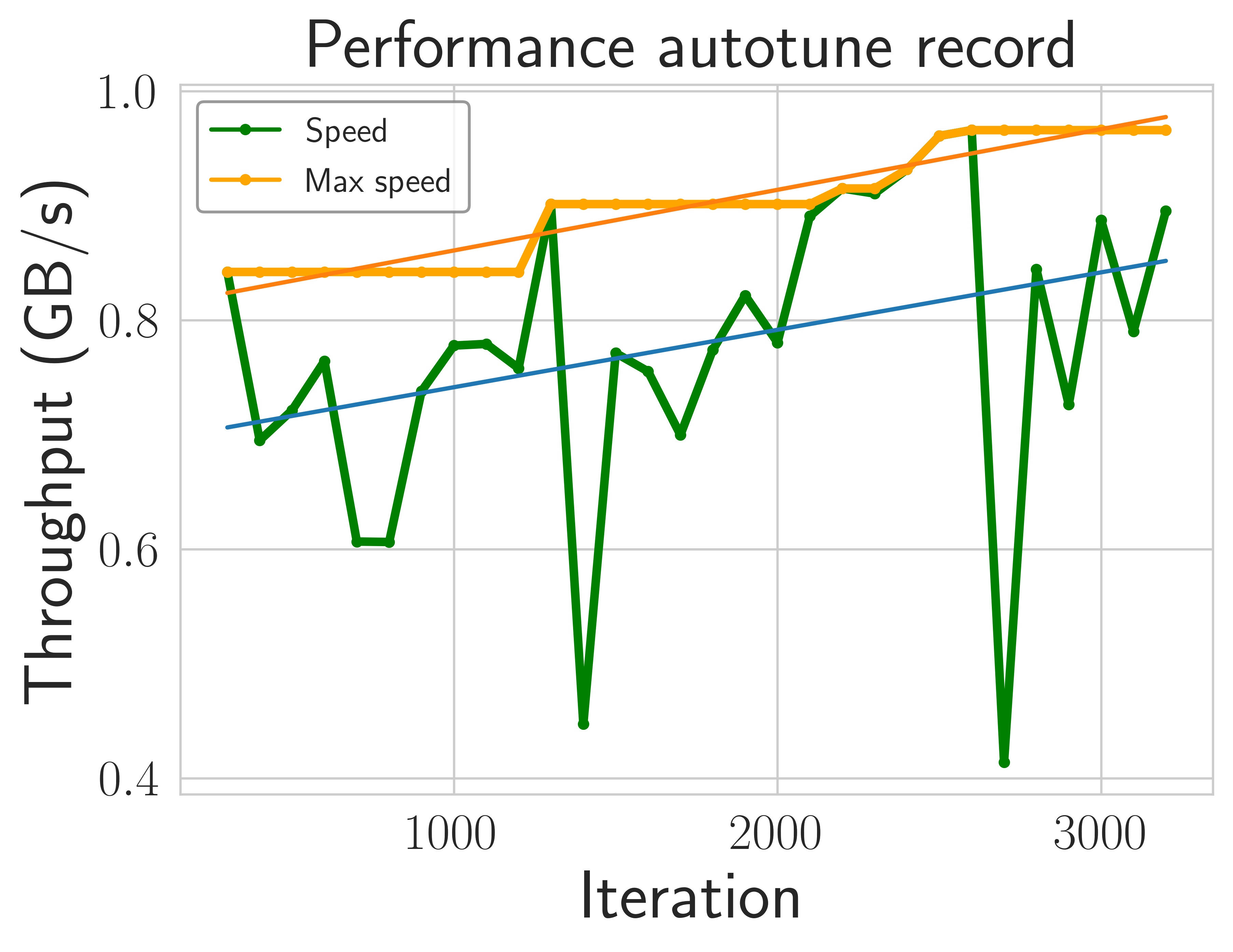
This figure shows the gradual increase in training performance during tuning. In this experiment, the hyperparameters are changed approximately every 100 iterations. The x-axis is the number of iterations. The y-axis is the data throughput.
Benchmark
Setup
We use up to 16 servers for benchmarks, each of which is equipped with 8 NVIDIA V100 32GB GPUs interconnected by NVLink. Servers are connected by 100 Gbps TCP/IP network. We compare the performance of Bagua with Horovod, PyTorch-DDP and BytePS on various tasks, including vision task (VGG16 on ImageNet), NLP task (BERT-Large finetune on SQuAD), and speech task (Transformer on AISHELL-2).
End-to-end performance
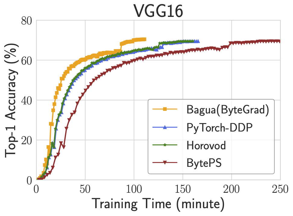
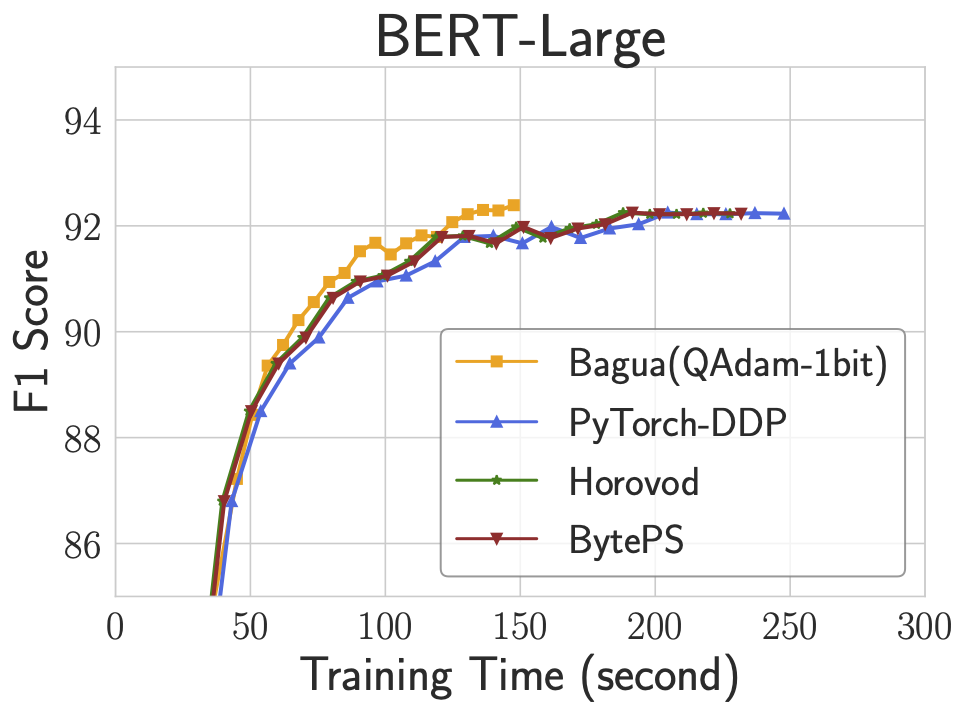
The figure above demonstrates the end-to-end training performance of three tasks. For each task, we select the best algorithm (according to the training efficiency and accuracy) from Bagua to compare with other systems. We use up to 128 GPUs (on 16 servers) to train three tasks:
- VGG16 on ImageNet with 128 GPUs; batch size per GPU: 32; Bagua algorithm: ByteGrad.
- BERT-Large Finetune on SQuAD with 128 GPUs; batch size per GPU: 6; Bagua algorithm: QAdam 1-bit.
- Transformer on AISHELL-2 with 64 GPUs; batch size per GPU: 32; Bagua algorithm: Decentralized.
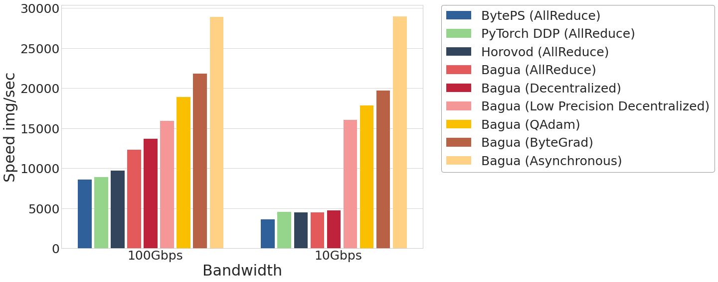
Scalability
VGG16 is known as a task that is difficult to scale because of its high ratio of communication and computation.
The following figure shows the training throughput for VGG16 on ImageNet with 128 GPUs under different network bandwidth. It also lists the performance of different built-in algorithms in Bagua.

Results show that Bagua can achieve multiple times of speedup compared with other systems.
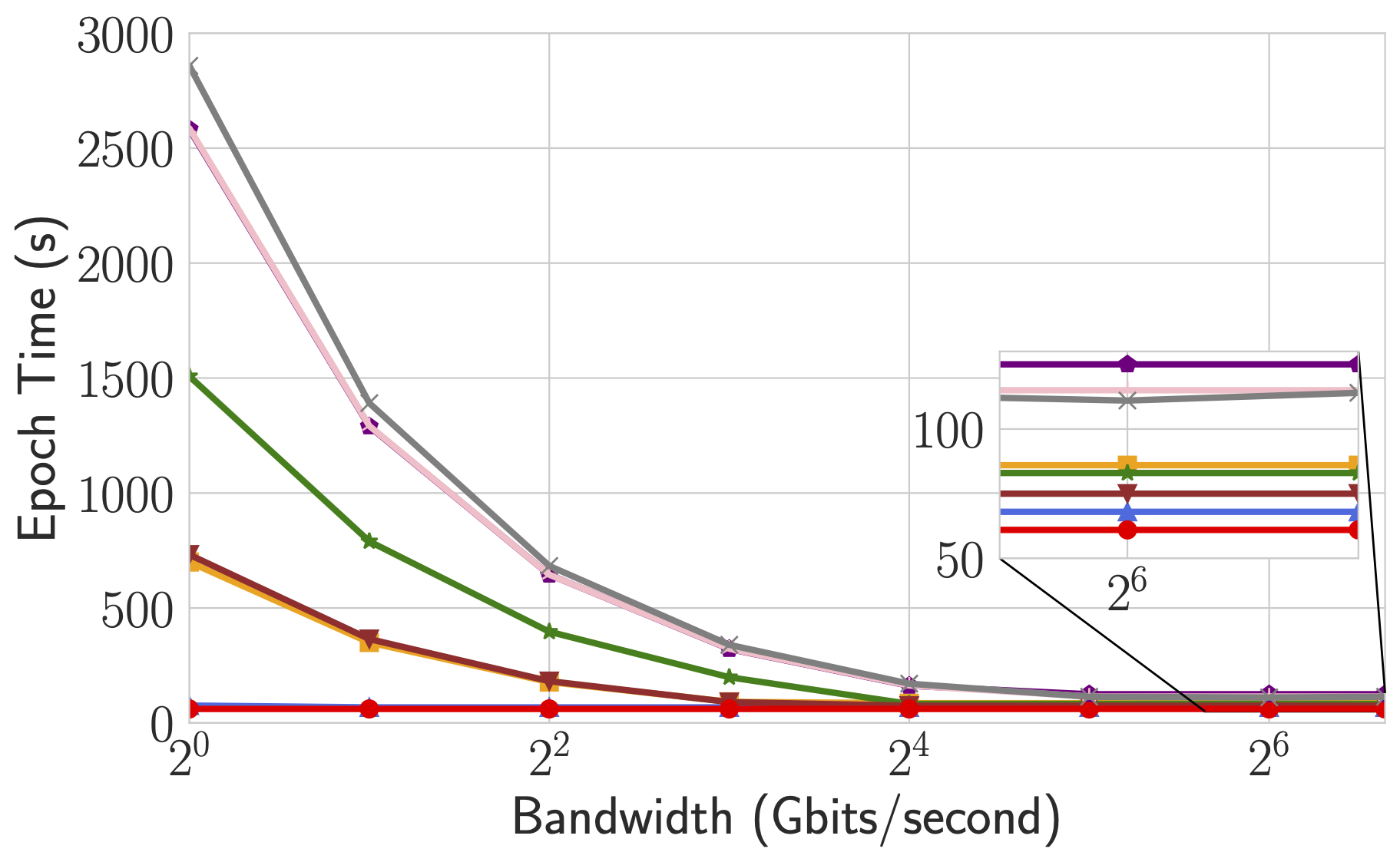
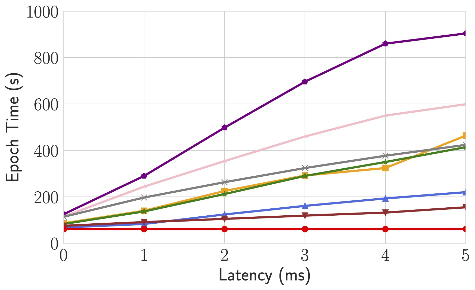
Trade-off of algorithms regarding network conditions
By supporting a diverse collection of algorithms, Bagua provides users the flexibility to choose algorithms for different tasks and network conditions (in terms of latency and bandwidth). To understand behaviors of these algorithms under different network conditions, we manually change the bandwidth and latency of connections between servers and report the epoch time accordingly.


This figure shows the epoch time of Bagua (with three algorithms) and other systems when the bandwidth has been changed from 100 Gbps to 1 Gbps, and the latency has been changed up to 5 ms. As we can see, when the interconnections are slower than the fast network that we previously adopted, Bagua can provide even more significant performance boost over the existing systems. Specifically, when the bandwidth is low, algorithms that require less amount of data transmission (e.g., QAdam, ByteGrad) outperform others. When the latency is getting high, algorithms that require fewer connections (e.g., decentralized SGD) tend to be degraded less than other methods. If we keep increasing the latency, we can observe that the decentralized SGD outperforms all others.
Elastic Training
Introduction
By applying TorchElastic, bagua can do elastic training. We usually use the capabilities of Elastic Training to support the following two types of jobs:
Fault tolerant jobs
Jobs that run on infrastructure where nodes get replaced frequently, either due to flaky hardware or by design. Or mission critical production grade jobs that need to be run with resilience to failures.
Dynamic capacity management
Jobs that run on preemptible resources that can be taken away at any time (e.g. AWS spot instances) or shared pools where the pool size can change dynamically based on demand.
Quickstart
You can find a complete example at Bagua examples.
1. Make your program recoverable
Elastic training means that new nodes will be added during the training process. Your training program need to save the training status in time, so that the new joining process can join the training from the most recent state.
For example:
model = ...
model.load_state_dict(torch.load(YOUR_CHECKPOINT_PATH))

for train_loop():
    ...
    torch.save(model.state_dict(), YOUR_CHECKPOINT_PATH)
2. Launch job
You can launch elastic training job with bagua.distributed.run. For example:
Fault tolerant (fixed number of workers, no elasticity)
python -m bagua.distributed.run \
        --nnodes=NUM_NODES \
        --nproc_per_node=NUM_TRAINERS \
        --rdzv_id=JOB_ID \
        --rdzv_backend=c10d \
        --rdzv_endpoint=HOST_NODE_ADDR \
        YOUR_TRAINING_SCRIPT.py (--arg1 ... train script args...)
Part of the node failure will not cause the job to fail, the job will wait for the node to recover.
HOST_NODE_ADDR, in form <host>[:<port>] (e.g. node1.example.com:29400), specifies the node and
the port on which the C10d rendezvous backend should be instantiated and hosted. It can be any
node in your training cluster, but ideally you should pick a node that has a high bandwidth.
If no port number is specified
HOST_NODE_ADDRdefaults to <host>:29400.
Elastic training(min=1, max=4)
python -m bagua.distributed.run \
        --nnodes=1:4 \
        --nproc_per_node=NUM_TRAINERS \
        --rdzv_id=JOB_ID \
        --rdzv_backend=c10d \
        --rdzv_endpoint=HOST_NODE_ADDR \
        YOUR_TRAINING_SCRIPT.py (--arg1 ... train script args...)
For this example, the number of training nodes can be dynamically adjusted from 1 to 4.
Reference
Kubernetes operator for Bagua jobs
Bagua supports kubernetes with a dedicated Bagua operator. This greatly simplifies deployments in modern computing cluster.
Prerequisites
- Kubernetes >= 1.16
Installation
Run the operator locally
git clone https://github.com/BaguaSys/operator.git
cd operator

# install crd
kubectl apply -f config/crd/bases/bagua.kuaishou.com_baguas.yaml

go run ./main.go
Deploy the operator
Install Bagua on an existing Kubernetes cluster.
kubectl apply -f https://raw.githubusercontent.com/BaguaSys/operator/master/deploy/deployment.yaml
Enjoy! Bagua will create resources in namespace bagua.
Examples
You can run demos in config/samples:
Static mode
"Static mode" means running the Bagua distributed training job with fixed number of nodes, and no fault tolerance.
kubectl apply -f config/samples/bagua_v1alpha1_bagua_static.yaml
Verify pods are running:
kubectl get pods

NAME                           READY   STATUS    RESTARTS   AGE
bagua-sample-static-master-0   1/1     Running   0          45s
bagua-sample-static-worker-0   1/1     Running   0          45s
bagua-sample-static-worker-1   1/1     Running   0          45s
Elastic mode
"Elastic mode" means running the Bagua distributed training job in elastic mode, which means the number of nodes can be dynamically adjusted, and the job is fault tolerant.
kubectl apply -f config/samples/bagua_v1alpha1_bagua_elastic.yaml
Verify pods are running
kubectl get pods

NAME                            READY   STATUS    RESTARTS   AGE
bagua-sample-elastic-etcd-0     1/1     Running   0          63s
bagua-sample-elastic-worker-0   1/1     Running   0          63s
bagua-sample-elastic-worker-1   1/1     Running   0          63s
bagua-sample-elastic-worker-2   1/1     Running   0          63s
Frequently Asked Questions and Troubleshooting
Dataloader sometimes hang when num_workers > 0
Add torch.multiprocessing.set_start_method("forkserver"). The default "fork" strategy is error prone by design. For more information, see PyTorch documentation, and StackOverflow.
Error when installing Rust
If you see some error like the message below, just clean the original installation record first by rm -rf /root/.rustup and reinstall.
error: could not rename component file from '/root/.rustup/toolchains/stable-x86_64-unknown-linux-gnu/share/doc/cargo' to '/root/.rustup/tmp/m74fkrv0gv6708f6_dir/bk'error: caused by: other os error.
Hang when running a distributed program
You can try to check whether the machine has multiple network interfaces, and
use command NCCL_SOCKET_IFNAME=network card name (such as eth01) to specify
the one you want to use (usually a physical one). Card information can be
obtained by ls /sys/class/net/.
NCCL WARN Reduce: invalid reduction operation 4
Bagua requires NCCL version >= 2.10 to support AVG reduction operation. If you encounter error NCCL WARN Reduce: invalid reduction operation 4 during training, you can run import bagua_core; bagua_core.install_deps() in your Python interpreter or the bagua_install_deps.py script to install latest libraries.
To check the NCCL version Bagua is using, run import bagua_core; bagua_core.show_version().
Model accuracy drops
Using a different algorithm or using more GPUs has similar effect as using a different optimizer, so you need to retune your hyperparameters. Some tricks you can try:
- Train more epochs and increase the number of training iterations to 0.2-0.3 times more than the original.
- Scale the learning rate. If the total batch size of distributed training is increased by times, the learning rate should also be increased by times to be .
- Performing a gradual learning rate warmup for several epochs often helps (see also Accurate, Large Minibatch SGD: Training ImageNet in 1 Hour).